 -- no spikes on estimating interval,
 -- the sample is contaminated with spikes.
The procedure of radiometer signal integration can be considered as a sort of reducing dimension of the initial sampling space, where the samples are the result of analog-to-digital conversion. As a result of this procedure the sampling space within the integrating interval gets reduced to a single sample, which reflects the signal mean estimation.
A variety of circumstances when one needs to select some optimal procedure of the signal estimation is usually splitted into three classical cases.
These cases are well described in the classical statistic literature and lead correspondingly to Bayes, parametric and nonparametric algorithm of the estimation obtaining. The third case is the most frequent if we are interested in getting reliable robust estimation.
Despite the variety of effects, which are responsible for building the radiometer signal statistic (Christiansen, Högbom 1988), the standard radiometer signal processing - low bandwidth filtration - leads to the "normalization" of the end signal statistic (Levin 1974). However the spikes influence disturbers the signal distribution making the "tails" heavier, comparing to normal distribution function.
The model of realization of such a process as a mixture of normal and Poisson processes is considered in Erukhimov's (1988) article. Given calculations, show that the estimation offset strongly depends on the jam intensity and could be very different depending on used estimation algorithm. Thus, there is a way to depress jams having a few sorts of estimation all together and choosing the best one (with the least offset), using some available prior information.
For the given model it seems to be enough to have the mean average and median estimation. The first one is the optimum for the normally distributed noise signal, the second one practically does not have an offset for a reasonable level of spikes contamination.
Thus, the optimal mean estimating procedure takes us to chose one of the two previously obtained estimation, what could be done by testing two hypotheses:
 -- no spikes on estimating interval,
 -- the sample is contaminated with spikes.

Before choosing the classification algorithm let us make some reasonable assumptions:
Only the first condition is the main one, the others just lead to some limitation in using the considered algorithm.
Analyzing the above assumptions one can choose the suitable classification algorithm based on p-state measure, such as "Nearest Neighbor" one (Patrick 1972), which, in particular, has been effectively used in real time feedback system (Ulyanov, Chernenkov 1983)
In our particular case the classification algorithm sounds like this:
when processing the window number k we choose from alternative![]() mean estimations that one which is closest to one chosen for window k-1.
mean estimations that one which is closest to one chosen for window k-1.
Applying the mentioned algorithm the following recursive formula can be written:

where:

The estimation is robust, because there is no dependency from signal distribution parameters, neither from spikes power involved. Because there is no need to increase sample amount for estimation calculation -- in opposite to Hodges-Lehmann algorithm, the meaning average and the median can be obtained fast enough.
Let us write down the steps of algorithm
Because of the obvious justifiability of the considered estimation and also continuity of the data acquisition process, for the real-time case one could take off the first step, using zero estimation mean instead.
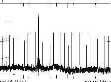
Tabl.1 contains the comparison of the processing results, obtained by described method on the first cabin "Continuous" data acquisition complex, with the previous ones. The significant performance benefit as compared to best rank estimations could be seen. There is also variance benefit as compared to other algorithm despite the greater spikes power level. The table contains the results of 60000 samples records processing. One of those records is shown in Figure 1.

Figure 1: The record, processed by different algorithms.
The quality of the considered algorithm could be also illustrated by Figure 2. At the top of the Figure the record containing the source and spike jams is drawn. The results of the different sorts of 5-time compression - of this record - meaning average, Hodges-Lehmann procedure, considered algorithm, - are drawn at the bottom. One could see the considered adaptive algorithm is preferable even by low degree of compression, because all spikes have been depressed.
:
The results of the 5-time compression of the model record by meaning
average, Hodges-Lehmann procedure and the considered algorithm.
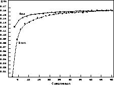
A disadvantage of the considered algorithm is the appearance of some extra correlation between subsequent samples in the output process. This effect is typical for any feedback algorithm acting as a low bandwidth filter. The dependence of the mentioned extra correlation on the compression factor, which is obtained by numerical modeling, is drawn in Figure 3.

Figure 3:
The dependency of subsequent samples correlation coefficient in compression
ratio.
The odd and even compression factor points are drawn as different curves. It
could be seen that there is slight increasing of correlation with increasing
of the compression ratio up to asymptotic value about  . Perhaps it could
be considered as a consequence of well known effect of dropping the
efficiency of median estimation to the asymptotic value
  with the increasing
the amount of samples (Hodges, Lehmann 1967).
Such a kind of relation to the features of median estimation could be also
confirmed by different means of the correlation coefficient for the odd and
even compression factor values.
Despite the fact the graph is obtained for the initial Gauss distribution of noise process, it actually does not have a strong dependence on the type of initial distribution, if the mentioned above assumptions are justified. That is because the output process gets normalized starting even from small averaging windows.
Thus, if the above mentioned condition are true, the extra correlation effect could be neglected at practical use of considered algorithm.
: The comparison of the processing results,
obtained by described method.